Welcome everyone. I would like to share my experience of building my own LLM from scratch. In this article, you will come across the details of LLM architecture. I followed a great book: Building Large Language Models (From Scratch) by Sebastian Raschka.
The whole point is that I built the GPT architecture piece by piece, layer by layer. Once done, it was impossible to train on the CPU/GPU I have locally, so I loaded the weights of GPT-2, which are publicly available from OpenAI. As the last part of the process, I also fine-tuned the model to solve classification problems like spam detection. The series will contain 2-3 articles – from building the GPT architecture to pre-training to fine-tuning.
The whole experience enriched my understanding of the deep inner workings of Large Language Models.
I will be adding some code snippets, which are just a glimpse of some aspects covered. You can skip those if not needed. They are optional and only serve to deepen understanding.
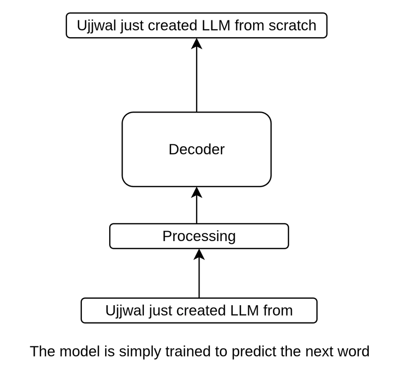
LLMs use a Decoder to predict the next word
Broadly speaking, the GPT architecture predicts the next word, which happens repeatedly. This iterative process generates entire new sentences, paragraphs, and even pages.

GPT-2 is an autoregressive, decoder-only model. Autoregressive models incorporate their previous outputs as inputs for future predictions.
How does it predict? The architecture will be explained step by step in the next sections.
Building text tokenisation
This layer maps discrete objects (here, texts) to points in a continuous vector space.
Tiktoken has a public dataset with token values for all the vocabulary in GPT-2. This was used to create the tokenising layer. Tokenisation is simply converting every vocabulary item into an ID, which is an integer number. A total of 50,257 tokens are used in GPT-2.

You can learn more about how byte-pair encoding is used to generate token IDs here: https://www.geeksforgeeks.org/nlp/byte-pair-encoding-bpe-in-nlp/
Building text embeddings
An embedding layer is created which converts the tokens into embeddings, each of 768 dimensions. The layer corresponds to two steps.
Step 1: A torch embedding layer is created with the input dimension equal to vocabulary size and output size of 768 (for GPT-2 small). This neural network layer is trained during pre-training (via backpropagation).

Step 2: A positional embedding is calculated and added to the token embedding to get the final vector embedding. The positional embedding has the same dimension as the token embedding. This is calculated by taking values [0,1,2,3…] and embedding them using a torch embedding layer.
token_embedding_layer = torch.nn.Embedding(vocab_size, output_dim)

positional_embedding_layer = torch.nn.Embedding(context_len, output_dim)
positional_embedding = positional_embedding_layer(torch.arange(context_len))

# Calculating vector embedding
input_embedding = token_embedding + positional_embedding

The attention mechanism is very important in LLMs. It allows each position in the input to consider the relevance of all other positions in a sequence.
You can learn more about attention mechanism basics here: https://www.ibm.com/think/topics/attention-mechanism.
In this implementation, a multi-head attention mechanism is coded. Multiple instances of self-attention are created, each with its own set of weights. The outputs are then combined. Multi-head attention is computationally expensive but very important for recognizing complex patterns.
Multi-head attention is also called Scaled Dot-Product Attention.

Multi-head attention mechanism implementation
You can read more about multi-head attention here: https://www.geeksforgeeks.org/nlp/multi-head-attention-mechanism/.
In GPT-2 small, there are 12 attention heads. So each output vector of a head has a dimension of output_dim (768) / num_heads (12).
The three weights—W_query, W_key, and W_value—are trained later via backpropagation.
Keys, queries, and values are obtained by splitting the input embeddings (which already include positional embeddings) into multiple heads. Then, the dot product is calculated for each head. Masking is applied before calculating the attention scores. Finally, the outputs of all heads are concatenated.

From the above diagram, you can see that future attention scores are masked, allowing the model to generate new, accurate, and sensible tokens.

The following softmax function is used for calculating attention scores:

This is how each attention score is calculated for each head:

Later, all the heads are concatenated to obtain the final query vector.
We have now created the multi-head attention mechanism. This is a core part of the GPT model.
In the next article, we will implement the transformer block and output layers before attempting to pre-train the model.
Here’s a summary of what we’ve done so far and what’s upcoming:

See you in the next article.