A Straightforward Guide for B+Trees

As a software engineer, adding an index is probably the most common fix when you hit a performance issue in your database. You’ve likely heard people say, “Just add an index, and the query will be much faster.” But have you ever wondered why that actually works?

In this article, we’ll explore what it really means to add an index and why it makes queries so much more efficient. I’ll keep everything as straightforward as possible.

Before we dive in, I’m assuming you have a basic understanding of data structures and algorithms, plus some familiarity with database management systems like MySQL or PostgreSQL. What we’re covering here isn’t specific to any particular DBMS. Instead, it’s a general concept that applies across the board, though each system might implement it a bit differently.

When you add an index to a database, you’re essentially creating a data structure behind the scenes. More specifically, the database creates something called a B+Tree.
Let’s say we have the following table:

ID | Name     | BadgeNumber (Index)
---|----------|--------------------
1  | Alice    | 1029 
2  | Bob      | 1856 
3  | Charlie  | 1735
4  | David    | 1021
5  | Emma     | 1069
6  | Frank    | 1035
7  | Grace    | 1280
8  | Henry    | 1002
9  | Ivy      | 1689
10 | Jack     | 1050
11 | Karen    | 1999
12 | Leo      | 1005
13 | Maria    | 2025
14 | Nathan   | 1120
15 | Olivia   | 1431
16 | Peter    | 1618
17 | Quinn    | 1008
18 | Rachel   | 1194

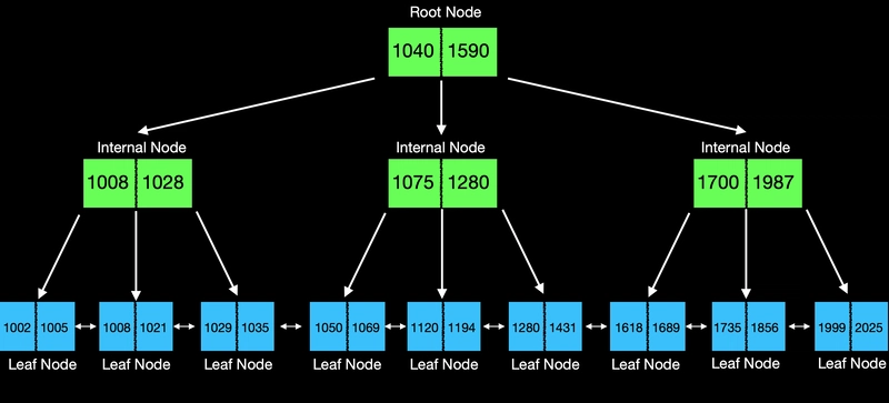
After adding an index on the BadgeNumber column, the database creates this B+Tree internally:

I know this might look intimidating at first—and that’s totally fine! We’ll break down exactly what a B+Tree is in just a bit. For now, here’s the key takeaway: when you create an index, the database builds a B+Tree data structure for you and uses it to find data incredibly quickly.

A B+Tree has two different types of nodes, and understanding the difference between them is key to understanding how the whole thing works.

Internal Nodes: The Navigation System

Think of internal nodes as your GPS—they guide you to where you need to go, but they don’t actually store your destination.

Here’s how they work:

• An internal node contains K keys and K+1 children (pointers)
• The keys act as boundaries that divide values into ranges
• The children point to either other internal nodes or leaf nodes

The root node is just a special internal node that happens to sit at the top—it doesn’t have a parent.

Let’s look at a concrete example. Suppose we have an internal node with 2 keys and 3 children:

(V represents the value of key)

Here’s what each child represents:

• ChildA (V < 1075): Points to all data with values less than 1075
• ChildB (1075 ≤ V < 1280): Points to all data with values from 1075 up to (but not including) 1280
• ChildC (v ≥ 1280): Points to all data with values of 1280 and above

Let’s say we’re searching for the value 1120. Here’s what happens:

1. First, we ask: “Is 1120 less than 1075?” No, so we skip ChildA
2. Next, we ask: “Is 1120 less than 1280?” Yes! So we follow ChildB

This guarantees that if the value 1120 exists anywhere in the tree, it must be somewhere in the subtree pointed to by ChildB.

Important note: Internal nodes don’t need to store actual data—they only need to store the right keys for navigation. If you look at the diagram above, you’ll notice that the key 1075 doesn’t actually exist as a record in the leaf nodes, while 1280 does. That’s perfectly fine! Internal nodes are just signposts, not data storage.

Leaf Nodes: The Data Warehouse

This is where the actual data lives. Each key in a leaf node represents a real record that exists in your database.
(Quick note: Different databases implement this slightly differently. For example, MySQL’s Innodb engine stores primary keys in leaf nodes and requires a second lookup to fetch the actual row data. For now, we’ll assume leaf nodes store the complete data—it’s simpler and covers the general concept.)

The big difference between leaf nodes and internal nodes is that all leaf nodes are linked together in a chain. Each leaf node points to its neighbors on both sides. This design makes range queries super efficient, which we’ll explore in detail later.
Here’s what it looks like:
Each leaf node stores actual data records and maintains pointers to its neighboring leaf nodes.

The Key Distinction

Here’s something crucial to understand:

• When you see the key “1280” in an internal node, it’s saying: “values of 1280 and above go this way.” It’s a signpost, nothing more. It doesn’t guarantee that a record with key 1280 actually exists.
• But when you see the key “1280” in a leaf node, it’s making a definitive statement: “Yes, there is absolutely a record with key 1280, and here it is—with all its data.”

Internal nodes guide you. Leaf nodes deliver.

B+Tree Property

Now that we’ve seen the structure, let’s talk about what makes B+Trees special. Don’t worry about memorizing these properties—they’ll all make perfect sense by the end of the article.

1. M-way tree: Multiple children per node

Each node in a B+Tree can have up to M children. In our diagrams above, M = 3, which means each node can have up to 3 children. This is what makes B+Trees “wide” rather than “tall”—and that’s a good thing for performance.

2. Perfectly balanced: Every path is the same length

In a B+Tree, every single search takes exactly the same number of steps, no matter what you’re looking for.

In our example, the distance from the root node to any leaf node is always 2 steps. Always. Whether you’re searching for 1050 or 1500, you take the same journey.

Even better? The tree stays balanced after insertions and deletions. This is probably the most important property of B+Trees because it guarantees that every search operation is consistently efficient. No worst-case scenarios where one search takes 10 times longer than another.

3. Key relationship: n keys means n+1 children

This is a simple rule that holds for all internal nodes: if a node has n keys, it must have exactly n+1 children.

In our diagrams, every internal node has 2 keys and 3 children (2+1). The keys create boundaries, and you need one more child than you have boundaries to cover all the ranges.

4. Sorted keys: Everything stays in order

Within each node, the keys are always sorted from smallest to largest. This makes searching incredibly efficient—you can use binary search within a node if needed, and you always know which direction to go.

Again, don’t stress about memorizing these. As we work through examples, you’ll see these properties in action and they’ll become second nature.

So far, we’ve talked about what an index is and broken down the structure of a B+Tree. But we haven’t answered the big question yet: Why does using a B+Tree make queries so much faster?

Let’s find out.

The Problem: Searching Without an Index

First, let’s go back to our simple table example and see what happens when we don’t have a B+Tree.

Imagine we want to find an employee whose badge number is 1320. Without an index, we’re stuck with sequential search—we have to check every single record, one by one, until we find it (or reach the end).

The time complexity? O(n), where n is the number of records in your table.

If you have 10 records, no big deal. But what about 10 million records? Now you’ve got a serious bottleneck. This is exactly why we need B+Trees.

The Solution: Searching With a B+Tree

The approach is simple: we compare our target value against the keys in each node, and whenever we find a key that’s greater than our target, we follow the pointer just before it. We keep going down until we reach a leaf node.

Let’s walk through finding badge number 1320 step by step:

1. At the root node (1040 | 1590)
   • We ask: “Is 1040 greater than 1320?” Nope, so we move to the next key.
   • We ask again: “Is 1590 greater than 1320?” Yes! So we follow the middle pointer down to the next level.
2. At the first level of internal node (1075 | 1280)
   • We ask: “Is 1075 greater than 1320?” No, so we move to the next key.
   • We ask: “Is 1280 greater than 1320?” Still no. Since there are no more keys to check, we follow the rightmost pointer down.
3. At the leaf node (1320 | 1431)
   • Now we’re at a leaf node—this is where the actual data lives!
   • We scan the keys and immediately find 1320. Done!

We found our target in just 2 steps down the tree. Compare that to potentially checking 18 records with sequential search.

That’s the power of B+Trees.

(Quick note: In real implementations, you could use binary search within each node to make things even faster. For now, I’m keeping it simple with linear search within nodes to make the logic crystal clear.)

Range Queries: Where B+Trees Really Shine

Before we dive into time complexity, let’s look at another type of search that shows off one of the B+Tree’s coolest features: range queries.

Suppose we want to find all employees with badge numbers between 1000 and 1200. How do we do that?

It’s actually surprisingly elegant. We use the same approach as a regular search to find the starting point (1000), and then we simply follow the leaf node pointers to scan through all the values in our range.

Let’s walk through it:

1. At root node (1040 | 1059)
   • We ask: “Is 1000 less than 1040?” Yes! So we follow the left pointer down.
2. At the first level of internal node (1008 | 1028)
   • We ask: “Is 1000 less than 1008?” Yes! So we follow the left pointer down again.
3. At the leaf node (1002 | 1005)
   • Now we’re at a leaf node. Instead of stopping, we start scanning sideways using the next pointer.
   • We move from leaf to leaf, collecting every value between 1000 and 1200, until we pass our upper bound.

This is where those leaf node pointers really prove their worth. Once we’ve navigated down to our starting point, we can scan through all the values in our range by simply following the linked list of leaf nodes—no need to go back up to the root and traverse down again for each value.

Without those pointers, we’d have to do a separate top-to-bottom search for every single value in the range. That would be painfully slow.

The Cost Of Search Operation

Now let’s see why exactly does using a B+Tree make queries so much faster?

Take a look at this diagram
Here’s the key insight: every time we move down one level, we eliminate a huge chunk of our search space.

Let’s trace through an example with 18 total records:

• At the root node: We’re starting with all 18 records as possibilities. Our search space is 18.
• At the second layer: By following one pointer, we’ve just eliminated 2/3 of the tree. Now our search space is only 6 records.
• At the leaf node level: We cut it down again by 2/3. Now we’re down to just 2 records to check.

See what’s happening? At each level, we’re dividing our search space by 3. That’s exponential reduction.

This is why the time complexity of searching in a B+Tree is O(log_k n), where:

• k = the maximum number of children a node can have
• n = the total number of records

The bigger k is, the fewer levels you need. And fewer levels means fewer steps.

Let’s make this concrete with realistic numbers.

Imagine a B+Tree storing 1 million records, where each node can hold 100 keys (which means 101 child pointers). How many steps does it take to find a specific record?

Let’s calculate:

Level 1 (Root):

• The root has 100 keys and 101 pointers
• It can point to 101 different subtrees

Level 2:

• We have at most 101 nodes at this level
• Each can hold 100 keys with 101 child pointers
• Total nodes at the next level: 101 × 101 = 10,201

Level 3:

• We have at most 10,201 nodes here
• Each points to 101 children
• Total possible leaf nodes: 10,201 × 101 = 1,030,301

Notice that 1,030,301 is greater than 1,000,000. This means we need exactly 3 levels to store one million records when each node holds 100 keys.

Mathematically, this is what log₁₀₁(1,000,000) ≈ 3 tells us.

To find any record among 1 million records:

• With B+Tree: 3 steps (worst case)
• With sequential scan: 1,000,000 steps (worst case)

This is why indexes are so powerful.

At this point, you might be wondering: “If each node has 100 keys, don’t we need to scan through those 100 keys at every level? Shouldn’t that count toward the cost?”

Great question! And the answer reveals something important about how databases actually work.

The reason we ignore scanning within nodes comes down to how databases physically store B+Trees—and it’s all about the massive speed difference between two types of operations:

1. Disk I/O (moving between levels): Slow and expensive
2. Memory operations (scanning within a node): Fast and cheap

Here’s what actually happens:

When you traverse from one level to another, the database needs to perform a disk access. In database terminology, it’s reading a “page” from disk into memory. This operation is significantly slow—we’re talking orders of magnitude slower than anything happening in RAM.

But once that data is loaded into memory? Scanning through the 100 keys in that node is blazingly fast. Plus, since the keys are sorted, we can even use binary search to make it even faster.

The simple summary is: Traversing down levels requires expensive disk I/O operations. Scanning through keys within a node only requires cheap in-memory operations.

That’s why when we talk about search cost in B+Trees, we only count the number of levels we traverse—not the scanning we do within each node. The disk I/O is the real bottleneck.

Searching is only half the story. Databases also need to insert new data—and when that happens, the B+Tree needs to adapt while maintaining its efficient structure.

Inserting data into a B+Tree follows a straightforward two-step process:

Step 1: Navigate to the right leaf node

We use the exact same search approach we learned earlier to find where the new value belongs. This ensures the value ends up in the correct position, maintaining the sorted order of the tree.

Step 2: Determine the insertion scenario

Once we’ve found the target leaf node, we check its capacity. How much room does it have? Based on the answer, we’ll face one of three possible scenarios, each requiring a different approach.

Before we dive into those scenarios, here’s what’s important to remember: no matter what happens during insertion, two properties must remain intact:

1. Perfect balance – Every path from root to leaf stays the same length
2. Sorted keys – Keys remain in order within every node

These properties are non-negotiable. They’re what guarantee that search operations stay fast and efficient, even as the tree grows and changes.

Now, let’s look at what actually happens when we insert…

Scenario 1: Simple Insertion (Leaf Has Space)

This is the easiest case. If the target leaf node isn’t full, we just insert the value and we’re done.

Let’s say we want to insert value 77 into this B+Tree:
(Quick note: You might notice some keys are missing in the node—that’s totally fine and happens in real B+Trees. As long as the tree maintains its core properties, it’s valid.)

We navigate down to the leaf node (68 | _ ) using our standard search approach. Since there’s one empty slot, we simply insert 77 into that node:
Done! No splitting, no restructuring—just a straightforward insertion.

Scenario 2: Leaf Split with Parent Having Space

But what if the leaf node is already full? Then we need to split it.

Let’s walk through an example. We want to insert value 80:

We navigate down to the target leaf node (68 | 77), and we immediately see a problem—it’s full.

The leaf node is full, so we have to split.

1. Insert the new value (80) in the correct sorted position: (68 | 77 | 80)
2. Split this full node into two separate leaf nodes:
   • Left node: (68 | 77)
   • Right node: (80 | _ )
3. Update the next pointers so the leaf nodes stay linked

Now we need to tell the parent about the new leaf node. We do this by copying the first key from the new right leaf node (80) up into the parent:
After this update, the parent now has three children with clear boundaries:

• Left child: All values < 35
• Middle child: All values from 35-80
• Right child: All values ≥ 80

The tree is now balanced again, and all keys remain sorted.

Scenario 3: Cascading Splits (Both Leaf and Parent Full)

Now for the tricky case: what if the parent is also full and can’t accommodate the new key we’re trying to copy up?

The answer: we recursively split upward until we either find a node with space or create a brand new root node.

Let’s see this in action. We want to insert value 100:

We navigate to the leaf node (99 | 118).

The leaf is full, so we split it just like before:

1. Insert 100 in sorted order: (99 | 100 | 118)
2. Split into two nodes: (99 | 100) and (118 | _)
3. Update the leaf pointers
4. Copy the first key (118) up to the parent

But wait—the parent is also full! So we need to split it too.

Splitting an internal node is similar to splitting a leaf, but with one key difference:

1. Insert the new key (118) in sorted order
2. Find the middle key
3. Push (not copy) the middle key up to the parent
4. Split the node around that middle key

Notice the difference: with leaf nodes, we copy the key up. With internal nodes, we push the key up, removing it from the current level.

In our case, the grandparent is also full. So we repeat the split process one more time, which creates a brand new root node:

We’ve successfully inserted our value, and the updates have cascaded all the way to the root.

The tree’s height increased by one level, but here’s what matters: all the critical properties remain intact:

• ✅ Perfectly balanced (all paths from root to leaf are the same length)
• ✅ Sorted keys (every node maintains sorted order)
• ✅ Proper structure (correct number of keys and children)

This is how B+Trees grow taller—from the bottom up, one split at a time.

Deleting a key from a B+Tree follows a similar high-level process to insertion:

1. Navigate to the leaf node containing the key
2. Delete the key from that node
3. Check if the node is now underflow

After deletion, a node might have too few keys or children—we call this “underflow.” Here’s when it happens:

• For leaf nodes: If the number of keys drops below K/2 (where K is the maximum number of keys)
• For internal nodes: If the number of children drops below (K+1)/2

When underflow occurs, we need to fix it to keep the tree efficient. We have two strategies:

Strategy 1: Redistribution (Borrowing)
We borrow a key (for leaf nodes) or a child (for internal nodes) from a sibling. But we can only do this if the sibling won’t underflow after lending us one.

Strategy 2: Merge
We combine two nodes into one. For this to work:

• Leaf nodes: The sum of keys from both nodes must be ≤ K
• Internal nodes: The sum of children from both nodes must be ≤ K+1

No matter which strategy we use, the B+Tree must remain valid—balanced, sorted, and properly structured.

Scenario 1: Deletion with Merge

Let’s say each node can hold at most 3 keys (K = 3). We want to delete the value 71.

We find the leaf node containing 71 and delete it:

Now the leaf node only has 1 key (68). That’s less than K/2 = 1.5, so we have underflow.

Let’s analyze our options:

• Redistribution? No. Both siblings have only 2 keys. If we borrow one, they’d have 1 key, causing them to underflow too.
• Merge? Yes! We can merge with either sibling. Let’s use the left sibling: (37 | 40) + (68) = 3 keys total, which fits perfectly.

Merge with left sibling
After merging, we notice the parent node now has an extra key. It has 2 children but 2 keys—it should only have 1 key for 2 children.

We remove the key 67 from the parent:
Done! The B+Tree is valid again, and we’ve successfully deleted key 71.

Scenario 2: Deletion with Redistribution

Same setup: K = 3. This time we want to delete key 71, but the tree looks a bit different:

We find and delete 71:

Again, underflow—the leaf node now has only 1 key. Let’s analyze our options:

• Redistribution? Yes! Both siblings have 3 keys. We can borrow one without causing them to underflow.
• Merge? No. Both siblings are full (3 values each), so merging would exceed our capacity.

Let’s borrow key 55 from the left sibling:
Here’s a problem: the parent still has key 67 as a boundary, but the first key in our leaf node is now 55. The boundary is incorrect!

We need to update 67 to 55 in the parent node. Remember, internal node keys are just boundaries—we need a value that’s ≤ the first key in the right subtree. So 55 works perfectly:
Perfect! The tree is valid and balanced.

Scenario 3: Cascading Merge (Shrinking the Tree)

One more example. K = 3, and we want to delete key 41.

We delete key 41 from the leaf:

Underflow again—the leaf has only 1 key. Let’s analyze leaf node options:

• Redistribution? No. Left siblings have 2 keys. Borrowing would cause it to underflow.
• Merge? Yes! We can merge with left sibling. Let’s merge with the left sibling: (22 | 29) + (37) = 3 keys.

Let’s merge with left sibling.

Now the parent is in trouble—it only has 1 child, but internal nodes need at least (K+1)/2 = 2 children. The parent is underflow!
Let’s analyze parent node options:

• Redistribution? No. The left sibling only has 2 children. Taking one would cause it to underflow.
• Merge? Yes! The sum of children is 1 + 2 = 3, which is ≤ K+1 = 4.

Let’s merge internal nodes.

Now we have a new merged internal node, but we need to figure out what key goes in the middle. We copy the first key (22) from the right leaf node up:
The root now has only 1 child—that’s underflow for an internal node. But the root is special: it has no siblings to borrow from or merge with.

The solution? Remove the root entirely:
The node (9 | 22 | _ ) becomes the new root. The tree’s height has shrunk by one level, but it’s still perfectly valid and balanced.

The Cost Of Update Operation

Now that we’ve walked through insertion and deletion, let’s talk about their performance cost.

The good news? The time complexity is very similar to search operations—O(log_k n).

Here’s why: every update (insert or delete) starts with searching for the right leaf node. Once we find it, we perform the update and might need to recursively adjust parent nodes if there’s overflow or underflow. But remember what we discussed earlier about disk I/O versus in-memory operations? Once the data is loaded into memory, these adjustments happen blazingly fast.

Update operations aren’t free, though. Everything we’ve discussed applies to one index. If your table has multiple indexes—say, five or six—every single insert or delete needs to update all of those B+Trees.

That’s why you might still face performance issues with massive insertions or deletions, even with indexes. Each index adds overhead. It’s a classic trade-off: indexes speed up reads but slow down writes.

We’ve covered a lot in this article. We started by asking what an index really is, broke down the structure of B+Trees, and saw exactly how they make queries so much faster.

Here’s the key takeaway: adding an index isn’t magic—it’s just creating a smart data structure that the database can use to find data quickly.

B+Trees are one of the most powerful data structures in computer science. They make finding records incredibly fast while guaranteeing the tree stays balanced after every insertion and deletion. That balance is what keeps performance consistent, no matter how much your data grows.

Of course, there’s always more to explore. We didn’t dive into B+Tree variants, composite indexes, or how different database systems like MySQL and PostgreSQL actually implement B+Trees under the hood. But I hope this article gives you a solid foundation—enough that you can confidently explore those topics on your own if you’re curious.

I’m not a database engineer—just a software engineer who loves learning and sharing what I’ve figured out. If you spot any mistakes or have suggestions, please let me know in the comments. I genuinely appreciate the feedback and want to make sure this is as accurate and helpful as possible.