Data Analysis & Visualization with Python: Bank Marketing Dataset Tutorial (Part 1)

Master Real-World Data Analysis Through a Complete Banking Case Study

Part 1 of 11: Introduction & Dataset Setup

If you’re looking to break into data analysis or sharpen your Python skills with real-world datasets, you’ve come to the right place. This comprehensive 11-part series will take you from raw data to actionable insights using a fascinating banking dataset.

What makes this series different? We’re not using toy datasets or simplified examples. Instead, you’ll work with actual marketing campaign data from a Portuguese bank, learning the exact workflows data analysts use in the industry every day.

🎯 What You’ll Learn in This Tutorial

By the end of this article, you’ll be able to:

Install and configure essential Python data analysis libraries
Fetch real-world datasets from the UCI Machine Learning Repository
Understand the structure and context of banking marketing data
Set up your environment for professional data analysis
Identify the business problem behind the data

Skill Level: Beginner to Intermediate

Time Required: 20-30 minutes

Prerequisites: Basic Python knowledge

🏦 The Business Problem: Understanding Bank Marketing Campaigns

Before diving into code, let’s understand what we’re analyzing and why it matters.

The Real-World Context

A Portuguese banking institution ran multiple direct marketing campaigns between 2008 and 2013, primarily through phone calls, to promote term deposit subscriptions to their clients.

What’s a term deposit? It’s a cash investment held at a financial institution for a fixed period with a guaranteed interest rate. Banks love these products because they provide stable, predictable funding.

The Challenge

Marketing campaigns are expensive. Each phone call costs time, money, and resources. The bank needed to answer a critical question:

Can we predict which clients are most likely to subscribe to a term deposit before we call them?

This is where data science transforms business operations. By identifying high-probability clients, the bank can:

Reduce costs by targeting the right customers
Increase conversion rates through focused efforts
Improve customer experience by reducing unwanted calls
Optimize resource allocation across campaigns

This type of predictive modeling is used across industries—from retail recommendations to healthcare risk assessment.

⚙️ Setting Up Your Python Environment

Let’s get your workspace ready for professional data analysis.

Step 1: Install Required Libraries

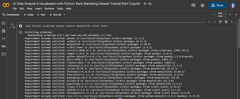
Open your Python environment (Jupyter Notebook, Google Colab, or VS Code) and run:

!pip install ucimlrepo pandas seaborn matplotlib scikit-learn

Get started quickly: https://colab.research.google.com/

New to colab?

Getting Started with Google Colab: A Beginner’s Guide

Understanding Each Library

ucimlrepo → Direct access to 600+ datasets from UCI Machine Learning Repository

pandas → The industry standard for data manipulation and analysis

seaborn → Statistical data visualization built on matplotlib

matplotlib → Core plotting library for creating custom visualizations

scikit-learn → Machine learning toolkit (we’ll use this in later parts)

Pro tip: If you’re using Google Colab, most of these libraries come pre-installed except ucimlrepo.

📦 Loading and Exploring the Dataset

Step 2: Import Your Libraries

from ucimlrepo import fetch_ucirepo
import pandas as pd
import seaborn as sns
import matplotlib.pyplot as plt

Step 3: Fetch the Bank Marketing Dataset

The UCI repository assigns each dataset a unique ID. For Bank Marketing, it’s ID 222:

# Fetch the dataset directly from UCI repository
bank_marketing = fetch_ucirepo(id=222)

This single line downloads 45,211 records of real banking data. The fetch_ucirepo object contains:

data.features → Independent variables (X)
data.targets → Dependent variable (y)
metadata → Dataset documentation
variables → Column descriptions and data types

Step 4: Create Your Working DataFrame

# Extract features and target
X = bank_marketing.data.features
y = bank_marketing.data.targets

# Combine into a single DataFrame for analysis
df = pd.concat([X, y], axis=1)

# Preview the first few rows
df.head()

Understanding the Data Structure

Your DataFrame now contains 17 columns:

Demographic Information:

age → Client’s age in years
job → Type of occupation (12 categories)
marital → Marital status
education → Education level

Financial Indicators:

balance → Average yearly balance in euros
housing → Has housing loan? (yes/no)
loan → Has personal loan? (yes/no)
default → Has credit in default? (yes/no)

Campaign Details:

contact → Contact communication type
month → Last contact month of year
duration → Last contact duration in seconds
campaign → Number of contacts performed during this campaign

Previous Campaign Data:

pdays → Days since client was last contacted (-1 means never contacted)
previous → Number of contacts before this campaign
poutcome → Outcome of previous marketing campaign

Target Variable:

y → Did the client subscribe? (yes/no) ← This is what we’re trying to predict

🔍 Dataset Intelligence: Metadata Analysis

Professional data analysts always start by understanding the dataset’s documentation.

# Display comprehensive metadata
print(bank_marketing.metadata)

Key Dataset Characteristics

Scale and Scope:

Total Records: 45,211 client interactions
Features: 16 predictor variables
Target Variable: Binary classification (subscribed: yes/no)
Time Period: 2008-2013
Geographic Location: Portugal

Data Quality Indicators:

Missing Values: Present in some categorical features (marked as “unknown”)
Data Type Mix: Numerical, categorical, and binary variables
Class Imbalance: Likely (most marketing campaigns have low conversion rates)

Business Context from Metadata

The dataset description reveals important details:

Multiple campaigns were conducted over several years
Phone calls were the primary contact method
Client history from previous campaigns is included
Economic indicators might influence subscription decisions

📊 Variable Dictionary: Understanding Each Column

# Examine variable details
bank_marketing.variables

Why This Matters

Understanding variable types is crucial for choosing the right analysis techniques:

Categorical Variables require encoding for machine learning

Numerical Variables need scaling and outlier detection

Binary Variables are already in usable format but may need balancing

Feature Categories Breakdown

Personal Attributes (4 features):

Demographics that don’t change frequently
Used to segment customer profiles

Economic Indicators (4 features):

Financial status metrics
Strong predictors of term deposit interest

Campaign Metrics (5 features):

Marketing effectiveness indicators
Reveal client engagement patterns

Historical Data (3 features):

Previous interaction outcomes
Often the strongest predictors in retention modeling

💡 Why This Dataset Is Perfect for Learning

For Beginners

✅ Clear business context → You understand the real-world application

✅ Well-documented → Every column has a clear explanation

✅ Manageable size → 45K rows is large enough to be realistic, small enough to process quickly

✅ Binary outcome → Easier to interpret than multi-class problems

For Intermediate Learners

✅ Mixed data types → Practice handling categorical and numerical variables

✅ Class imbalance → Learn to deal with skewed target distributions

✅ Feature engineering opportunities → Create derived variables from existing ones

✅ Real business metrics → Understand how data drives business decisions

For Career Development

✅ Portfolio-worthy project → Demonstrate end-to-end analysis skills

✅ Interview-ready topic → Discuss classification problems confidently

✅ Industry-relevant → Marketing analytics is a high-demand field

✅ Transferable skills → Apply these techniques to any classification problem

🎓 Practice Exercises: Hands-On Learning

Before moving to Part 2, strengthen your understanding with these exercises:

Exercise 1: Data Structure Exploration

# What are the dimensions of your dataset?
df.shape

# What data types does each column have?
df.info()

# What are the basic statistics for numerical columns?
df.describe()

What to look for:

How many rows and columns do you have?
Which columns are numerical vs categorical?
What are the ranges of numerical variables?

Exercise 2: Missing Value Detection

# Count missing values per column
df.isnull().sum()

# Calculate the percentage of missing values
(df.isnull().sum() / len(df)) * 100

Critical thinking questions:

Which columns have missing data?
What might “unknown” values represent?
How might missing data affect your analysis?

Exercise 3: Target Variable Distribution

# Check the balance of your target variable
df['y'].value_counts()

# Visualize the distribution
df['y'].value_counts().plot(kind='bar')
plt.title('Target Variable Distribution')
plt.xlabel('Subscribed to Term Deposit?')
plt.ylabel('Count')
plt.show()

Business insight question:

What does this distribution tell you about the campaign’s success rate?

🚀 What’s Coming in Part 2

Now that you’ve successfully loaded and understood the dataset, we’ll dive deeper into data exploration:

Part 2: Understanding Data Structure & Quality Assessment

You’ll learn:

Advanced techniques for detecting data quality issues
How to identify outliers and anomalies
Data type conversion and optimization
Creating your first data quality report
Best practices for documenting your findings

📚 Additional Resources

Want to dive deeper?

💬 Join the Conversation

Working through this tutorial? I’d love to hear about your experience:

What challenges did you encounter?
What insights did you discover in the data?
What would you like to see covered in future parts?

Drop a comment below or connect with me to discuss data analysis techniques!

🔖 Series Navigation

You are here: Part 1 – Introduction & Dataset Setup

Next: Part 2 – Understanding Data Structure & Quality Assessment

Coming soon: Parts 3-11 covering EDA, visualization, modeling, and deployment

Follow me for the complete 11-part series on data analysis and visualization. Each article builds on the previous one, creating a comprehensive learning path from raw data to actionable insights.

#DataScience #Python #MachineLearning #DataAnalysis #BankingAnalytics #PredictiveModeling #PythonProgramming #DataVisualization #UCI #CareerDevelopment

About the Author: A developer who loves learning and sharing diverse tech experiments — today’s focus: making sense of data with Python.

Source link