
Have you ever wondered how your music, voice calls, or even video streams travel from the physical world into the digital devices we use every day? The answer lies in signal processing the art of converting an analog signal into a digital one.
In this post, I’ll walk you through a simple MATLAB simulation where I generate an analog sine wave, sample it, quantize it, and finally encode it into binary form. By the end, you’ll see how an analog signal transforms step by step into a digital stream.
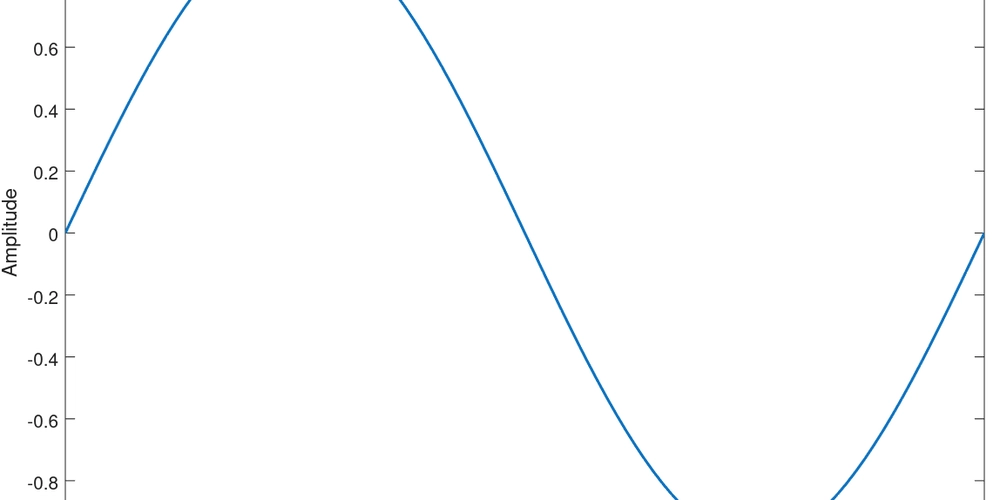
1. Generating an Analog Signal
Let’s start with a simple sine wave of 100 Hz. Since MATLAB doesn’t truly handle “continuous” signals, I approximate it with a very fine time step:
t = 0:0.0001:0.01;       % very fine step (continuous-like time)
f = 100;                 % frequency = 100 Hz
x_analog = sin(2*pi*f*t);

plot(t, x_analog, 'LineWidth', 1.5);
title('Analog Signal (Sine Wave)');
This gives me the smooth curve — my reference signal.
2. Sampling
According to the Nyquist theorem, I need to sample at least twice the frequency of the signal (≥ 200 Hz).
I tested three cases:
- 150 Hz (below Nyquist) → aliasing and distortion
- 200 Hz (at Nyquist) → minimal capture, jagged
- 500 Hz (above Nyquist) → clean sampling, closer to analog
Fs = 500;   % try 150, 200, and 500
Ts = 1/Fs;
n = 0:Ts:0.01;
x_sampled = sin(2*pi*f*n);

stem(n, x_sampled, 'filled');
title(['Sampled Signal at Fs=" num2str(Fs) " Hz']);
3. Quantization
Next, I map the sampled values to discrete amplitude levels. Using more bits increases the number of levels:
- 8 bits → 256 levels
- 16 bits → 65,536 levels
- 64 bits → practically continuous
bits = 8;   % try 8, 16, and 64
levels = 2^bits;
x_min = min(x_sampled);
x_max = max(x_sampled);
q_step = (x_max - x_min)/levels;

x_index = round((x_sampled - x_min)/q_step);
x_quantized = x_index*q_step + x_min;

stem(n, x_quantized, 'filled');
title(['Quantized Signal (' num2str(bits) '-bit)']);
With fewer bits, you can clearly see stair-step distortions. As I increase the bits, the quantized signal becomes almost identical to the sampled one.
4. Encoding
Finally, each quantized value is represented as a binary word. For example, with 8 bits, each sample becomes an 8-bit binary code.
binary_codes = dec2bin(x_index, bits);
disp(binary_codes(1:10,:));   % first 10 codes
When concatenated, they form a digital bitstream — the format that computers and communication systems love.
Points
- If you sample below Nyquist, you risk losing information (aliasing).
- Increasing sampling rate improves signal quality but costs more data.
- More quantization bits reduce distortion, but increase storage and bandwidth.
- At the end, your “smooth” analog wave becomes a long sequence of 1s and 0s.
You can try experimenting with different frequencies and bit depths in your own code. It’s the best way to see how analog signals become digital and to appreciate the balance between accuracy and efficiency in real-world systems.